A Lack of Context

What I wish source systems would tell us and they hardly ever do. Best laid out as an example, look at this data:

𝟺𝟻𝟽𝟾𝟸𝟷, 𝟹 𝟶𝟶𝟶, 𝟸𝟶𝟸𝟶-𝟶𝟿-𝟸𝟶

This alone does not tell us much, so along with this we need context, commonly in the form of column names:

𝙲𝚄𝚂𝚃𝙾𝙼𝙴𝚁 𝙽𝚄𝙼𝙱𝙴𝚁, 𝙱𝙰𝙻𝙰𝙽𝙲𝙴, 𝚃𝙸𝙼𝙴𝚂𝚃𝙰𝙼𝙿

Fine, this is usually all we get. Now, let’s shake things up a bit by introducing a second line of data. Now we have:

𝟺𝟻𝟽𝟾𝟸𝟷, 𝟷𝟼 𝟶𝟶𝟶, 𝟸𝟶𝟸𝟶-𝟶𝟿-𝟸𝟶
𝟺𝟻𝟽𝟾𝟸𝟷, 𝟹 𝟶𝟶𝟶, 𝟸𝟶𝟸𝟶-𝟶𝟿-𝟸𝟶

Confusing, but this happens. Is the timestamp not granular enough and these were actually in succession? Is one a correction of the other? Can customers have different accounts and we are missing the account number?

Even if you can get all that sorted out, we can shake it up further. Put this in a different context:

𝙿𝙰𝚃𝙸𝙴𝙽𝚃 𝙽𝚄𝙼𝙱𝙴𝚁, 𝚁𝙰𝙳𝙸𝙰𝚃𝙸𝙾𝙽 𝙳𝙾𝚂𝙴, 𝚃𝙸𝙼𝙴𝚂𝚃𝙰𝙼𝙿

Now I feel the need to know more. Are these measurements made by different persons and how certain are they? What is the margin of error? If these were in succession, what were their durations? If only one of them is correct, which one is it?

More sources should communicate data as if it was a matter of life and death. This is what Transitional modeling is all about.

Tinker, Tailor, Raspberry Pi

I went ahead and got myself a Raspberry Pi 4B with 4GB RAM, which I intend to use as a job scheduling server, only to find out that the suggested OS, Raspberry Pi OS, is 32-bit. Fortunately, the Linux distro Alpine, which I’ve grown very fond of lately, is available for Raspberry Pi as aarch64, meaning it’s both 64-bit kernel and userland. Unfortunately the distro is currently, as of version 3.12, not set up for persistent storage and is more of a live playground. Gathering bits and pieces from various guides online, this can however be remedied with some tinkering. In this article you will find how to set up a persistent 64-bit OS on the Raspberry Pi, share a USB attached disk, while also adding some interesting software.

If you go ahead and buy the Pi 4, note that it has micro-HDMI ports. I thought they were mini, for which I already had cabling, but alas, another adapter had to be purchased. Also, when attaching a USB disk it is better if it is externally powered. The Pi can however power newer external SSD drives that have low power consumption. I tried with a magnetic disk based one powered over USB first, but it behaved somewhat strangely. With that said, let’s go ahead and look at how to get yourself a shiny tiny new server.

Tinkering for Persistence

After downloading the v3.12 tarball from Alpine on my macOS, it’s time to set up the SDHC card for the Pi. I actually borrowed my old hand-me-down MacBook Air that I gave to my daughter a few years ago, since it has a built-in card reader, as opposed to my newer Air. The Pi boots off a FAT32 partition, but we want the system to reside in an ext4 partition later, so we will start by reserving a small portion of the card for the boot partition. This is done using Terminal in macOS with the following commands.

diskutil list
diskutil partitionDisk /dev/disk2 MBR "FAT32" ALP 256MB "Free Space" SYS R
sudo fdisk -e /dev/disk2
> f 1
> w
> exit

The tarball should have decompressed once it hit your download folder. If not, use the option “xvzf” for tar.

cd /Volumes/ALP
tar xvf ~/Downloads/alpine-rpi-3.12.0-aarch64.tar
nano usercfg.txt

The newly created file usercfg.txt should contain the following:

enable_uart=1
gpu_mem=32
disable_overscan=1

The least amount of memory for headless is 32MB. The UART thing is beyond me, but seems to be a recommended setting. Removing overscan gives you more screen estate. If you intend to use this as a desktop computer rather than a headless server you probably want to allot more memory to the GPU and enable sound. Full specification for options can be found on the official Raspberry Pi homepage.

After that we just need to make sure the card is not busy, so we change to a safe directory and thereafter eject the card (making sure that any pending writes are finalized).

cd
diskutil eject /dev/disk2

Put the SDHC card in the Pi and boot. Login with “root” as username and no password. This presumes that you have connected everything else, such as a keyboard and monitor.

setup-alpine

During setup, select your keymap, hostname, etc, as desired. However, when asked where to store configs, type “none”, and the same for the apk cache directory. If you want to follow this guide to the point, you should also select “chrony” as the NTP client. The most important part here though is to get your network up and running. A full description of the setup programs can be found on the Alpine homepage.

apk update
apk upgrade
apk add cfdisk
cfdisk /dev/mmcblk0

In cfdisk, select “Free space” and the option “New”. It will suggest using the entire available space, so just press enter, then select the option “primary”, followed by “Write”. Type “yes” to write the partition table to disk, then select “Quit”.

apk add e2fsprogs
mkfs.ext4 /dev/mmcblk0p2
mount /dev/mmcblk0p2 /mnt
setup-disk -m sys /mnt
mount -o remount,rw /media/mmcblk0p1

Ignore the warnings about extlinux. This and the following trick was found in the Alpine Wiki, but in some confusing order. 

rm -f /media/mmcblk0p1/boot/*
cd /mnt
rm boot/boot
mv boot/* /media/mmcblk0p1/boot/
rm -Rf boot
mkdir media/mmcblk0p1
ln -s media/mmcblk0p1/boot boot

Now the mountpoints need fixing, so run:

apk add nano
nano etc/fstab

If you prefer some other editor (since people tend to become religious about these things) then feel free to use whatever makes you feel better than nano. Add the following line:

/dev/mmcblk0p1   /media/mmcblk0p1   vfat   defaults   0 0

Now the kernel needs to know where the root filesystem is.

nano /media/mmcblk0p1/cmdline.txt

Append the following at the end of the one and only line in the file:

root=/dev/mmcblk0p2

After exiting nano, it’s safe to reboot, so:

reboot

After rebooting, login using “root” as username, and the password you selected during setup-alpine earlier. Now you have a persistent system and everything that is done will stick, as opposed to how the original distro was configured.

Tailoring for Remote Access

OpenSSH should already be installed, but it will not allow remote root login. We will initially relax this constraint. Last in this article is a section on hardening where we again disallow root login. If you intend to have this box accessible from the Internet I strongly advice on hardening the Pi.

nano /etc/ssh/sshd_config

Uncomment and change the line (about 30 lines down) with PermitRootLogin to:

PermitRootLogin yes

Then restart the service:

rc-service sshd restart

Now you should be able to ssh to your Pi. The following steps are easier when you can cut and paste things into a terminal window. Feeling lucky? Then now is a good time to disconnect your keyboard and monitor.

Keeping the Time

If you selected chrony as your NTP client it may take a long time for it to actually correct the clock. Since the Pi does not have a hardware clock, it’s necessary to have time corrected at boot time, so we will change the configuration such that the clock is set if it is more than 60 seconds off during the first 10 lookups. 

nano /etc/chrony/chrony.conf

Add the following line at the bottom of the file.

makestep 60 10

Check the date, restart the service, and check the (now hopefully corrected) date again.

date
rc-service chronyd restart
date

Having the correct time is a good thing, particularly when building a job scheduling server.

Silencing the Fan

Together with the Pi I also bought a fan, the Pimoroni Fan Shim. According to reviews it is one of the better ways to cool your Pi, but it’s still too soon for me to have an opinion. Unless controller software is installed, it will always run at full speed. It’s not noisy, but still noticeable sitting a metric meter from the Pi. Again, some tinkering will be needed since the controller software needs some prerequisites installed. We lost nano between reboots, so we will go ahead and add it again.

apk update
apk upgrade
apk add nano

Other software we need is in the “community” repositories of Alpine. In order to active that repository we need to edit a file:

nano /etc/apk/repositories

Uncomment the second line (ending in v3.12/community), exit, then install the necessary packages.

apk update
apk add git bash python3 python3-dev py3-pip py3-wheel build-base

After those prerequisites are in place, install the fan shim software using:

git clone https://github.com/pimoroni/fanshim-python
cd fanshim-python
./install.sh

apk add py3-psutil
cd examples
./install-service.sh

The last script will fail with “systemctl: command not found”, since Alpine uses OpenRC as its init system, and not systemd which this script presumes. We will instead write our own startup script:

nano /etc/init.d/fanshim

This new file should have the following contents:

#!/sbin/openrc-run

name="fanshim"
command="/usr/bin/python3 /root/fanshim-python/examples/automatic.py"
command_args="--on-threshold 65 --off-threshold 55 --delay 2"
pidfile="/var/run/$SVCNAME.pid"
command_background="yes"

There are a lot of interesting options for fanshim that you can explore, like tuning it’s RGB led. Now we want this to run at boot time, so add it the the default runlevel, then start it.

rc-update add fanshim default
rc-service fanshim start

Enjoy the silence!

Adding and Sharing a Disk

Some of files we will be transferring are going to be quite large. It would also be neat to be able to access files easily from the Finder in macOS, so I am adding a USB3 connected hard disk with 4TB storage. What follows will be very similar to setting up a NAS, and in fact, the way I fell in love with Alpine was by building my own NAS from scratch (with the minor differences being more disks and using zfs). 

First we need to change the filesystem. The disk comes formatted as FAT32, which is very poorly suited for a networked disk. Samba, which is what we will be using for sharing, more or less requires a filesystem that supports extended attributes. After plugging in the drive, we will therefore repartition the drive and format it to ext4. 

cfdisk /dev/sda

Using cfdisk, delete any existing partitions and create one new partition. It should become “Linux filesystem” by default. Don’t forget to “Write” before “Quit”. Then format it:

mkfs.ext4 /dev/sda1

Now we need to add autofs to get automatic mounting. This package is in edge/testing though, so we need to enable that branch and repository, but still have main and community take preference. This can be done by labelling a repository.

nano /etc/apk/repositories

Change the line with the testing repository (last line in my file) to the following. Note that yours will have some server.from.setup/path depending on what you selected in setup-alpine. You only uncomment and add the @testing label in other words.

@testing http://<server.from.setup/path>/edge/testing

Now autofs can be installed from the labelled repo.

apk add autofs@testing

Note that dependencies are still pulled from main/community to the extent it is possible. In order to configure autofs, first:

nano /etc/autofs/auto.master

Add the following line after the uncommented line starting with /misc. It will also disconnect the hard disk after 5 minutes to save energy:

/-   /etc/autofs/auto.hdd   --timeout=300

Then create this new config file:

nano /etc/autofs/auto.hdd

Add the the following line to the empty file.

/hdd   -fstype=ext4   :/dev/sda1

Now, the user pi needs to be created.

adduser pi
smbpasswd -a pi

Select desirable passwords for the pi user. The latter one will later be stored in the macOS keychain and therefore easy to forget, so make note of it somewhere. 

Add autofs to startup and start it now. Change the ownership of /hdd to pi.

rc-update add autofs default
rc-service autofs start
chown -R pi.pi /hdd

With that in place (disk can be accessed through /hdd) it is time to set up the sharing. For this we will use samba and avahi for network discovery.

apk add samba avahi dbus
nano /etc/samba/smb.cfg

Now, this is what my entire smb.cfg file looks like, with all the tweaks to get stuff running well from macOS.

[global]

  create mask = 0664
  directory mask = 0775
  veto files = /.DS_Store/lost+found/
  delete veto files = true
  nt acl support = no
  inherit acls = yes
  ea support = yes
  security = user
  passdb backend = tdbsam
  map to guest = Bad User
  vfs objects = catia fruit streams_xattr recycle
  acl_xattr:ignore system acls = yes
  recycle:repository = .recycle
  recycle:keeptree = yes
  recycle:versions = yes
  fruit:aapl = yes
  fruit:metadata = stream
  fruit:model = MacSamba
  fruit:veto_appledouble = yes
  fruit:posix_rename = yes 
  fruit:zero_file_id = yes
  fruit:wipe_intentionally_left_blank_rfork = yes 
  fruit:delete_empty_adfiles = yes 
  server max protocol = SMB3
  server min protocol = SMB2
  workgroup = WORKGROUP    
  server string = NAS      
  server role = standalone server
  dns proxy = no

[Harddisk]
  comment = Raspberry Pi Removable Harddisk                     
  path = /hdd    
  browseable = yes          
  writable = yes            
  spotlight = yes           
  valid users = pi       
  fruit:resource = xattr 
  fruit:time machine = yes
  fruit:advertise_fullsync = true

Those last two lines can be removed if you are not interested in using the disk as a Time Machine backup for your Apple devices. I will likely not use it, but since this is how I configured my NAS and it was a hassle to figure out how to get it working I thought I’d leave it here for reference. Doesn’t hurt to keep it there in any way.

Let us also configure the avahi-daemon, by creating a config file for the samba service. Avahi will announce the server using Bonjour, making them easily recognizable from macOS (where they automagically show up in the Finder). 

nano /etc/avahi/services/samba.service

This new file should have the following contents:

<?xml version="1.0" standalone='no'?>
<!DOCTYPE service-group SYSTEM "avahi-service.dtd">
<service-group>
<name replace-wildcards="yes">%h</name>
<service>
<type>_smb._tcp</type>
<port>445</port>
</service>
<service>
<type>_device-info._tcp</type>
<port>0</port>
<txt-record>model=RackMac</txt-record>
</service>
<service>
<type>_adisk._tcp</type>
<txt-record>sys=waMa=0,adVF=0x100</txt-record>
<txt-record>dk0=adVN=HDD,adVF=0x82</txt-record>
</service>
</service-group>

Not that the txt-record containing adVN=HDD can be removed if you are not interested in using the disk as a Time Machine backup. Still, leaving it won’t hurt.

Finally, it’s time to add samba and avahi to the startup and start the services.

rc-update add samba default
rc-update add avahi-daemon default
rc-service samba start
rc-service avahi-daemon start

The disk should now be visible from macOS. Remember to click “Connect as…” and enter “pi” as the username and your selected smbpasswd from earlier. Check the box “Remember this password in my keychain” for quicker access next time. Sometimes, due to a bug in Catalina, you may get “The original item cannot be found” when accessing the remote disk. If that happens, force quit Finder, and you should be good to go again. If anyone knows of any other fix to this issue, let me know!

Automation

Now, this server will be used as a job server. Some of the jobs running will need the psql command from PostgreSQL and some others will be R jobs. Let’s install both, or whatever you need to satisfy your desires. The dev and headers are needed when R wants to compile packages from source code. You can skip this step for now if you are undecided about what to run or just need basic services like the built-in shell scripting. However, in order to run programs as different users within Cronicle, sudo is necessary.

apk add R R-doc postgresql
apk add R-dev postgresql-dev linux-headers libxml2-dev 
apk add sudo

In order to automate these jobs, we will be using Cronicle. It depends on node.js so we need to install the prerequisites. It’s run script is fetched using curl, so it will also need to be installed.

apk add nodejs npm curl

The installation is done as follows (it is a oneliner even if it looks broken here).

curl -s https://raw.githubusercontent.com/jhuckaby/Cronicle/master/bin/install.js | node

I want to use standard ports, so I need to change the config slightly.

nano /opt/cronicle/conf/config.json

Change base_app_url from port 3012 to 80. Much further down, change http_port from 3012 to 80, and https_port from 3013 to 443. If you want mails to be sent, change smtp_hostname in the beginning of the file to the mail relay you are using. After that an initialization script needs to be run.

/opt/cronicle/bin/control.sh setup

Now we just need to get it running at boot time. This is, however, a service that we do not want to “kill” using a PID, so we are going to enable local scripts that start and stop the service in a controlled manner instead.

rc-update add local default
nano /etc/local.d/cronicle.start

This new file should have the following line in it:

/opt/cronicle/bin/control.sh start

Now we need to create a stop file as well:

nano /etc/local.d/cronicle.stop

This file should have the contents:

/opt/cronicle/bin/control.sh stop

In order for the local script daemon to run these, they need to be executable.

chmod +x /etc/local.d/cronicle.*

With that, let’s secure things.

Hardening

Now that most configuring is done, it’s time to harden the Pi. First we will install a firewall with some basic login protection using the builtin ‘limit’ in iptables. Assuming you are in the 192.168.1.0/24 range, which was set during setup-alpine, the following should be run. Only clients on the local network are allowed access to shared folders.

apk add ufw@testing
rc-update add ufw default
ufw allow 22
ufw limit 22/tcp
ufw allow 80
ufw allow 443
ufw allow from 192.168.1.0/24 to any app CIFS
ufw allow Bonjour

With the rules in place, it’s time to disallow root login over ssh, and make sure that only fresh protocols are used.

nano /etc/ssh/sshd_config

Change the line that previously said yes to no, and add the other lines at the bottom of the file (borrowed from this security site):

PermitRootLogin no

PrintMotd no
Protocol 2
HostKey /etc/ssh/ssh_host_ed25519_key
HostKey /etc/ssh/ssh_host_rsa_key
KexAlgorithms curve25519-sha256@libssh.org,diffie-hellman-group-exchange-sha256
Ciphers chacha20-poly1305@openssh.com,aes256-gcm@openssh.com,aes128-gcm@openssh.com,aes256-ctr,aes192-ctr,aes128-ctr
MACs hmac-sha2-512-etm@openssh.com,hmac-sha2-256-etm@openssh.com,umac-128-etm@openssh.com,hmac-sha2-512,hmac-sha2-256,umac-128@openssh.com

After that, enable ufw and restart sshd. Note that if something goes wrong here you will need to plug in a monitor and keyboard again to login locally and fix things.

ufw enable
rc-service sshd restart

Now is a good time to reboot and reconnect to check that everything is working.

reboot

With root not being able to login, you will instead login as “pi”. It is possible for this user to (temporarily, until exit) elevate privileges by the following command:

su

Another option is to use sudo, but I will leave it like this for now, and go ahead with setting up some jobs. That’s a story for another article though.

I hope this guide has been of help. It should be of use for anyone tinkering with Alpine on their Raspberries, and likely some parts for those running other Linux flavors on different hardware as well.
She’ll wear a grue dress

This is a continuation of the articles “She wore a blue dress” and “Rescuing the Excluded Middle“, which introduced crisp imprecision and fuzzy uncertainty. The former being evaluative and the latter both subjective and contextual. The articles discuss, relate, and sometimes further the formalization of transitional modeling, so they are best read with some previous knowledge of this technique. An introduction can be found starting with the article “What needs to be agreed upon” or by reading the scientific paper “Modeling Conflicting, Unreliable, and Varying Information“. In this article I will discuss the effect of a chosen language upon the modeling of posits, with particular homage to the new riddle of induction and Goodman’s predicate ‘grue’.

In order to look at the intricacies of using language to convey information about the real world, we will focus on the statement “She’ll wear a grue dress”. First, this refers to a future event, as opposed to the previously investigated statement “She wore a blue dress”, which obviously happened in the past. There are no issues talking about future events in transitional modeling. Let’s say Donna is holding the dress and is just about to put it on. She would then, with absolute certainty, assert the posit “She’ll wear a grue dress”. It may be the case that the longer time before the dress will be put on, the less certain Donna will be, but not necessarily. If she just after New Year’s Eve is thinking of what to wear at the next, she could still be certain. Donna could have made it a tradition to always wear the same dress.

There is a difference between certainty and probability. If Donna is certain she will wear that dress at the next New Year’s Eve, she is saying her decision has already been made to wear it, should nothing prevent her from doing so. From a probabilistic viewpoint, lots of things can happen between now and New Year preventing that from ever happening. The probability that she will wear the dress at next New Year’s Eve is therefore always less than 1, and will be so for any prediction. Assuming the probability could be determined, it would also be objective. Everyone should be able to come up with the same number. Bella, on the other hand, could be certain that Donna will not wear the dress at the next New Year’s Eve, since she intends to ruin Donna’s moment by destroying the dress. Certainty is subjective and circumstantial. I believe this distinction between certainty and probability is widely overlooked and the concepts confused. “Are you certain? Yes. Is it probable? No” is a completely valid and non-contradictory situation.

With no problems of talking about future events, let’s turn our attention to ‘grue’. Make note of the fact that you would not have reacted in the same way if the statement had been “She’ll wear a blue dress”, unless you happen to be among the minority already familiar with the color grue. If you belong to that minority, having studied philosophy perhaps, then forget for a minute what you know about grue. I will look at the word ‘grue’ from a number of different possibilities, of only the last will be Goodman’s grue.

What is grue?

  1. It is a color universally and objectively distinguishable from blue.
  2. It is a color selectively and subjectively indistinguishable from blue.
  3. It is a synonym of blue.
  4. It is an at the current time widely known color.
  5. It is an at the current time little known color.
  6. It is an at the current time unknown color that will become known.
  7. It is an at the current time known color synonymous with blue that at some point in the future will be considered different from blue (Goodman).

In (1) there will likely be no issues whatsoever. Perhaps there is a scientific definition of ‘grue’ as a range of wavelengths in between green and blue. On a side note and right now, the color greige is quite popular and a mix between grey and beige. Using that definition of ‘grue’ anyone should be able to reach the same conclusion whether an actual color can be said to be grue or not. Of course most of us do not possess spectrophotometers or colorimeters, so we will judge the similarity on sight. If enough reach the same conclusion, we may say it’s as close to an objectively determinable color as we will get. This is good, and not much thought has to go into using >grue< in a posit.

In (2) there may be potential issues. Perhaps grue and blue become indistinguishable under certain conditions, such as lighting, or let’s assume that 50% of the population cannot distinguish between grue and blue because of color blindness. Given two otherwise identical dresses of actual different colors, grue and blue, they may assert that she wore or will wear both of these, simultaneously. Such assertions can be made in transitional modeling and possible contradictions found using a formula over sums of certainty (see the scientific paper). To resolve this, non-contradiction either needs to be enforced at write time or periodically analyzed. Unknown types of color blindness could even be discovered this way, through statistically significant contradictory opinions. That being said, one should document already known facts and new findings with respect to effects that may disturb the objectivity of the values used.

In (3) there is a choice or a need for documentation. Either one of ‘blue’ and ‘grue’ is chosen and used consistently as the value or both are used but the fact that they are synonymous is documented. This may be a more common situation than one first may think, since ‘grue’ could be the word for ‘blue’ in a different language. This then raises the question of synonymy. What if there are language-specific differences between the interpretations of ‘grue’ and ‘blue’, so that they nearly but not entirely overlap? If grue allows a bit more bluegreenish tones than blue then they are only close to synonymous. This speaks for keeping values as they were stated, but that values themselves then may need their own model.

With those out of the way, let us look at how well known of a color grue is. In (4) almost everyone has heard of and use grue when describing that color. This is good, both those who are about to assert a posit containing >grue< will know how to evaluate it, and those later consuming information stored in posits will understand what grue is. With (5) difficulties may arise. In the extreme, I have invented the word ‘grue’ myself and nobody else knows about it. However, when interrogated by the police to describe the dress of the woman I saw at the scene of the crime, I insist on it being grue. No other color comes close to the one I actually saw. Rare values, like these, that likely can be explained in more common terms need translation. If done prescriptively the original statement is lost, but if not, it must be done descriptively at the cost of the one consuming posits first digesting translation logic. This is a very common scenario when reading information from some system, in which you almost inevitably find their own coding schemes, like “CR”, “LF”, “TX”, and “RX” turning out to have elaborate meanings.

Now (6) may at first glance seem impossible, but it is not. Let us assume that we believe the dress is blue and the posit temporally more qualified to “She’ll wear a blue dress on the evening of December 31st 2020”. Donna asserts this with 100% certainty the day after the preceding New Year’s Eve. When looking at the dress on December 31st 2020, Donna has learnt that there is a new color named grue, and there is nothing more fitting to describe this dress. Given this new knowledge, that the dress is and always has been grue, she retracts her previous posit, produce a new posit, and asserts this new one instead. The process can be schematically described as:

posit_1     = She'll wear a blue dress on the evening of December 31st 2020

assertion_1 = Donna, posit_1, 100% certainty, sometime on January 1st 2020

assertion_2 = Donna, posit_1, 0% certainty, earlier on December 31st 2020

posit_2     = She'll wear a grue dress on the evening of December 31st 2020

assertion_3 = Donna, posit_2, 100% certainty, earlier on December 31st 2020

Given new knowledge, you may need to correct yourself. This is precisely how corrections are managed in transitional modeling, in a bi-temporal solution, where it is possible to deduce who knew what when. This works for rewriting history as well:

posit_3     = The dress is blue since it was made on August 20th 2018

assertion_4 = Donna, posit_3, 100% certainty, sometime on August 20th 2018

assertion_5 = Donna, posit_3, 0% certainty, earlier on December 31st 2020

posit_4     = The dress is grue since it was made on August 20th 2018

assertion_6 = Donna, posit_4, 100% certainty, earlier on December 31st 2020

The dress is and always has been grue, even if grue was unheard of as a color in 2018. Nowhere do the posits and assertions indicate when grue started to be used though. This would, again be a documentation detail or alternatively warrant explicit modeling of values.

Finally there is (7), in which there is a point in time, t, before which we believe everything blue to be grue and vice versa. Due to some new knowledge, say some yet to be discovered quantum property of light, those things are now split into either blue or grue to some proportions. This is really troublesome. If some asserters were certain “She wore a blue dress” and others were certain “She wore a grue dress”, in assertions made before t, that was not a problem. They were all correct. After that point in time, though, there is no way of knowing if the dress was actually blue or grue from those assertions alone. If we are lucky enough to get hold of the dress and figure out it is blue, things start to look up a bit. We would know which asserters were wrong. Their assertions could be invalidated, while we make new ones in their place. In the less fortunate event that the dress is nowhere to be found, previous assertions could perhaps be downgraded to certainties in accordance with the discovered proportions of blue versus grue.

The overarching issue here, which Goodman eloquently points out, is that this really messes up our ability to infer conclusions from inductive reasoning. How do we know if we are in a blue-is-grue situation soon to become a blue-versus-grue nightmare? To me, the problem seems to be a linguistic one. If blue and grue have been used arbitrarily before t, but after t signify a meaningful difference between measurable properties, then reusing blue and grue is a poor choice. If, on the other hand, blue and grue were actually onto something all along, then this measurable property must have been present and in some way sensed, and many assertions likely to be valid nevertheless. This reasoning is along the lines of philosopher Mark Sainsbury, who stated that:

A generalization that all A’s are B’s is confirmed by instances unless we have good reason to believe that there is some property, O, such that every A-instance is O, and if those A-instances had not been O, they would not have been B.

In other words, some additional property is always hiding behind issue number (7).

With all that said, there are a lot of subtleties concerning values, but most, if not all of them can be sorted out using posits and assertions, with the optional addition of an explicit model of values, together with prescriptive or descriptive measures. That being said, if language is used with proper care and with the seven types of ‘grue’ mentioned above in mind, you will likely save yourself a lot of headaches. We also learnt that people normally think in certainties rather than probabilities.

Rescuing the Excluded Middle

This is a continuation of “She wore a blue dress“, in which we introduced to the concepts of imprecision and uncertainty. I will now turn the focus back on the imprecise value ‘blue’ and make that imprecision a bit more formal. In the works of Brouwer related to intuitionism an imprecise value can be thought of as a mapping. I will introduce the notation >blue< for such a mapping of the imprecise value ‘blue’. The mapping >blue< would then be:

>blue< : x ⟶ [0,1]

In other words, for any color x it evaluates to either 1 for it being fully considered as blue or 0 if it cannot be considered blue. However, according to Brouwer any value in between is also allowed. It could be 0.5 for half blue, which is also known as a fuzzy impecise value. Allowing these will confuse the with imprecision codependent concept of uncertainty. I will therefore restrict imprecise values, such as blue to:

>blue< : x ⟶ {true, false}

The reasoning is that subjectivity enters already in the evaluation of this mapping. In the terminology of transitional modeling, it is when asserting the statement “She wore a blue dress” that the asserter evaluates the actual color of the dress against the value ‘blue’. As such, the posit will be crisp from the asserter’s point of view. Given that the dress was acceptably ‘blue’ enough, the asserter can determine their certainty towards the posit. Values can therefore be said to be crisp imprecise values, but only relative a subject.

If we assume that the occasion when she wore a dress took place on the 1st of April 2020 and this is used as the appearance time in the posit, then it is also an imprecise value. Most of us will take this as the precise interval from midnight to midnight on the following day. At some point in that crisp interval, the dress was put on. Even so, putting on a dress is not an instantaneous event and time cannot be measured with infinite precision, so regardless of how precisely that time is presented, appearance time will remain imprecise.

With finer detail, the appearance time could, for example have been expressed as at two minutes to midnight on the 1st of April 2020. But, here we start to see the fallacy of taking some time range for granted though. With the same reasoning as before we would assume that to refer to the interval between two minutes and one minute to midnight. However, there is no way of knowing that a subject will always interpret it this way. So, we need the mapping once again:

>two minutes to midnight on the 1st of April 2020< : x ⟶ {true, false}

It seems as if the evaluation of this mapping is not only subjective, but also contextual. If we know that it could have taken more than a minute to put on the dress in question, then maybe this allows for both tree and one minute to midnight evaluating to true. Even when such a range is possible to specify it is almost never available in the information we consume, so we often have to deal with evaluations like these. We have, however, become so used to evaluating the imprecision that we do so more or less subconsciously.

But, didn’t we lose a whole field of applicability in the restriction of Brouwer’s mapping? That fuzziness is actually not all lost. I believe that what assertions do in transitional modeling is to fill that gap, while paying respect to subjectivity and contextuality. It is not possible to capture the exact reasoning behind the assertion, but we can at least capture its result. Recall that an assertion is someone expressing a degree of certainty towards a posit, here exemplified by “She wore a blue dress”. An example of an assertion is: “Archie thinks it likely that she wore a blue dress”. With time involved this becomes: “On the 2nd of April Archie thinks it likely that she wore a blue dress two minutes to midnight on the 1st of April”. Even more precisely and closer to a formal assertion: “Since the >2nd of April< the value >likely< appears for (Archie, certainty) in relation to ‘since the >1st of April< the value >blue< appears for (she, dress color)'”.

As can be seen, assertions can themselves be formulated as posits. Given the example assertion, it’s value is also imprecise, with a mapping:

>likely< : x ⟶ {true, false}

We have however, in transitional modeling, decided that certainty is better expressed using a numerical value. Certainty is taken from the range [-1, 1], with 1 being 100% certain, -1 being 100% certain of the opposite, and 0 for complete uncertainty. Certainties in between represent beliefs to some degree. We have to ask Archie, when you say ‘likely’, how certain is that given as a percentage? Let’s assume it is 80%. That means the corresponding mapping becomes:

>0.8< : x ⟶ {true, false}

Certainty is just another crisp imprecise value, but relative a subject who has performed a contextual evaluation of the imprecise values present in a posit with the purpose of judging their certainty towards it. An asserter (the subject) made an assertion (the evaluation and judgement), in transitional modeling terminology.

The interesting aspect of crisp imprecise values are that they respect “tertium non datur”, which is Latin for “no third is given”, more commonly known as the law of the excluded middle. In propositional logic it can be written as (P ∨ ¬P), basically saying that no statement can be both true and not true. An asserter making an assertion, evaluating whether the actual color of the dress can be said to be blue, obeys this law. It can either be said to be blue or it cannot. This law does not hold for fuzzy imprecise values. If something can be half blue, then neither “the dress was blue” nor “the dress was not blue” is fully true.

Fuzziness is not lost in transitional modeling though. Since certainty is expressed in the interval [-1, 1], it encompasses that of fuzzy values. The difference is that fuzziness comes from uncertainty and not from imprecision. Uncertainty is subjective and contextual, whereas fuzzy imprecise values are assumed objective and universal. I believe that this makes for a richer and truer to life, albeit more complex, foundation. It also rescues the excluded middle. Statements are either true or false with respect to crispness, but it is possible to express subjective doubt. Thanks to the subjectivity of doubt, contradicting opinions can be expressed, but that is the story of my previous articles, starting with “What needs to be agreed upon“.

As a consequence of the reasoning above, a posit is open for evaluation with respect to its imprecisions. Such imprecisions are evaluated in the act of performing an assertion, but an assertion is also a posit. In other words, the assertion is open for evaluation with respect to its imprecisions (the >certainty< and >since when< this certainty was stated). This can be remedied by someone asserting the assertion, but then those assertions will remain open, so someone has to assert the new assertions asserting the first assertions. But then those remain open, so someone has to assert the third level assertions asserting the second level assertions asserting the first level assertions, and so on…

Rather than having “turtles all the way down“, in transitional modeling there are posits all the way down, but for practical purposes it’s likely impossible to capture more than a few levels. The law of the excluded middle holds, within a posit and even if imprecise, but only in the light of subjective asserters performing contextual evaluations resulting in their judgments of certainty. To some extent, the excluded middle has been rescued!

Identification, identity, and key

Since we have started to recognize “keys” in our information modeling tool (from version 0.99.4) I will have this timely discussion on identification and identity. Looking at my previously published articles and papers, I have repeatedly stated that identification is a search process by which circumstances are matched against available data, ending in one of two outcomes: an identity is established or not. What these circumstances are and which available data you have may vary wildly, even if the intent of the search is the same. Think of a detective who needs to find the perpetrator of a crime. There may have been strange blotches of a blue substance at the crime scene, but no available register to match blue blotches of unknown origin to. We have circumstances but little available data, yet often detectives put someone behind bars nevertheless.

On the other hand, think of a data integrator working with a data warehouse. The circumstance is a customer number and you have a neat and tidy Customer concept with all available data in your data warehouse. The difference to the detective is the closeness of agreement between different runs of the identification process. The process will look very much the same for the next customer number, and the next, and the next. So much so that the circumstance itself may warrant its own classification, namely being a “key” circumstance. In other words, a “key” is when circumstances exist that every time produce an identical search process against well defined and readily available data. As such, a “key” does not in any way imply that it is the only way to identify something, that it is independent of which time frame you are looking at it, or that it cannot be replaced at some point.

These are the reasons why, in Anchor and Transitional modeling, no importance has been given to keys. Keys cannot affect a model, because if they did, the model itself would reflect a single point of view, be bound to a time frame, and run the risk of becoming obsolete. That being said, if a process is close to perfectly reproducible, it would be stupid not to take advantage of that fact and help automate it. This is where the concept of a “key” is useful, even in Anchor and Transitional modeling, which is why we are now adding it as an informational visualization with the intent of also creating some convenient functionality surrounding them. Even so, regardless of which keys you add to the model, the model is always unaffected by these, precisely for the reasons discussed above.

I hope this clarifies my stance on keys. They are convenient for automation purposes, since they help the identification process, but shall never affect the model upon which they work in any way.

Visualization of Keys

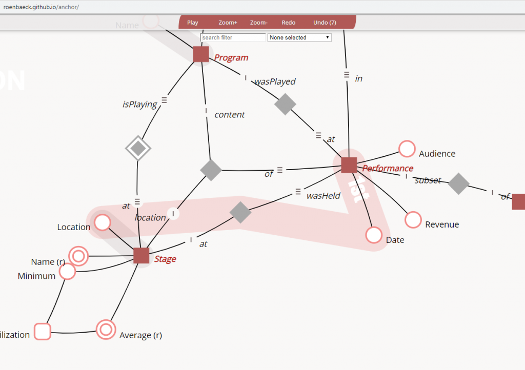
Visualization and editing of keys has been added in version 0.99.4 (test) of the free online Anchor modeling tool. This is so far only for informational purposes, but is of great help when creating your own automation scripts. Note that a key in an Anchor model behaves like a bus route, stopping on certain items in the graph. In order to create a key, select an anchor and at least one attribute (shift-clicking lets you do multiple select). To edit a created key, click on its grey route to highlight it red. You can then add or remove items or change it’s name. Click again to leave key editing mode. Along with this come some improvements to the metadata views in the database, and among them the new _Key view.

Time is both one and many

As you intuitively know, there is only one time. Yet in the domain of information modeling we speak of “valid time”, “transaction time”, “user defined time”, “system time”, “application time”, “happening time”, “changing time”, “speech act time”, “inscription time”, “appearance time”, “assertion time”, “decision time” and so on, as not being the same. In fact, I will boldly say that the only one of these coming close to true time is happening time, defined in Anchor modeling as ‘the moment or interval at which an event took place’, even if it goes on to define other types of time. However, if we assume that only happening times exist, then all other types of time should be able to be represented on the form:

[EventTimepoint].

In Transitional modeling we have the concept of a posit, with its appearance time defined as ‘the time when some value can be said to have appeared (or will appear) for some thing or a collection of things’. However, it also has assertion time, defined as ‘the time when someone is expressing an opinion about their certainty toward a posit’. To exemplify, “Archie and Bella will be ‘married’ on the 1st of April” and “Charlie is expressing that he is almost certain of this on the 31st of March”. In this case the 1st of April is the appearance time and 31st of March the assertion time.

Given the previous assumption on how to represent everything as events and time points, we can rewrite the previous example as [The value ‘married’ appears for Archie and Bella1st of April] and [The value ‘almost certain’ is given to a posit by Charlie31st of March]. Now they are on the same form, indicating that there is indeed only one true time. Why, then, do we feel the need to distinguish between appearance and assertion time? Why not just have a single “event time”? Well, as it turns out, there is a crucial difference between the two, but it has less to do with time and more to do with the actual events taking place.

Some events are temporally orthogonal to each other. Charlie can change his mind about how certain he is of the posit, independently of the posit itself. The posit “Archie and Bella will be ‘married’ on the 1st of April” remains the same, even if Charlie changes his mind and [The value ‘quite uncertain’ is given to a posit by Charlie1st of April]. Maybe Charlie realized that he may have been the subject of an elaborate prank, strengthened by the fact that he was only given one day’s notice of the wedding and that pranks are quite frequent on this particular day. To summarize, for one given point in appearance time there are now two points in assertion time. This means assertion time runs orthogonal to appearance time. They are two different “dimensions” of time.

But, really, there is only one time. We choose to view these as two dimensions, not because there are different times, but because there are different types of events. Plotting these on a plane just makes it easier for us to illustrate this fact. In Transitional modeling, assertion time is not only orthogonal to appearance time, it is also relative the one making the assertion. Let’s introduce Donna and [The value ‘absolute prank’ is given to a posit by Donna31st of March]. In other words, Donna knew from the start that the wedding was a prank. Now, for one given point in appearance time there are three points in assertion time, two belonging to Charlie and one belonging to Donna, with one also coinciding. Even so, there is only one time, but different and subjective events.

If these temporally orthogonal events are abundant, even the list of types of time presented in the beginning of the article may seem few. The problem is that we are used to seeing only one objective assertion time coinciding with the appearance time. Looking at the representation on a (helpfully constructed) plane, this would be the 45 degree line on which a (helpfully positioned) bitemporal timepoint has the same value for both its coordinates: (tx, ty) with tx ty. Most information, likely wrongfully, is represented on this line. We have lost the nuance of distinguishing between the actual information and the opinion of the one stating it. This makes it easy to fall into the trap thinking that there is no need to distinguish between orthogonal events. I have, unfortunately, seen many a database in which attempts have been made to crush orthogonal events into a single column with less than desirable results and the negative impact discovered in irrecoverable retrospect.

I believe that every new modeling technique, and any modeler dealing with time in existing techniques, must decide on which events it wants to recognize as important and if they are temporally orthogonal or not. If not, they will never be able to represent information close to how information behaves in reality. Orthogonal events will need different timelines and different timelines need to be managed separately, such as being stored in different columns or tables in a database. I think there are many orthogonal events of interest, some quite generally applicable and some very specific to certain use cases. While we could get away with a single “event time” we often choose not to. The reasoning is that by making orthogonal events integral to a modeling technique allows for it to provide their theory, stringency, consistency and optimization.

Recognizing orthogonal events can therefore be a smart move. The events of interest in Transitional modeling is “the appearance of a value” and “having an opinion”. The events of interest in the works of Richard T. Snodgrass are “making a database fact valid in the modeled reality”, “making a database fact true in the database”. The events of interest in the works of Tom Johnston are “entering a certain state”, “utterances about enterings of states”, and “the inscription of utterances”, and so goes on for all modeling techniques. We have all probably added to the confusion, but if we can start to recognize a common ground and that we only slightly differ in the events we recognize, this terminological mess can be untangled. With all the notions afloat, the question that begs answers is what events you recognize and if any of them are subjective? Feel free to share in the comments below!

I do think it’s time for all of us to abide by the thought of one true time, dissociated by temporally orthogonal events, and be careful when using the misleading ‘dimensions of time’ notion.

When what if is if what

I created my first data mining model back in 2005. This was a basket analysis in which we determined which products are commonly found together (numerous connection) and which are almost never found apart from each other (strong connection). We used this to rearrange the shelves in five stores, putting the numerously connected products in corners of the store, driving as many people past other shelves as possible. Strongly connected products were kept in the same or adjoining shelves. This increased the upsell of about 30%, so shortly after the evaluation, all 900 stores were rebuilt according to the new layout.

Ever since then, I’ve been in awe of what data mining, now often referred to as machine learning, can do. I am sure many of you have employed and maybe even operationally use such models. Having continued to use them to score customers, from churn likelihood to cross sales potential to probability of accepting an offer and to many other things, I sat down in 2013 and wondered what the next step could be. Here I was at a company with several well working models, but even though they were labeled as “predictive”, none could acutally tell me much about the future. So I started thinking; What if there was a way to hook up the models to the cash flow?

As it turns out, there was a way. So far, the models had been used to more or less categorize customers, such as in “potential churners” and “loyal customers”, based on some threshold of the probability to churn. However, behind the strict categorization are individual probabilities for churn. Even loyal customers have a probability to churn, albeit a low one. The first realization was that if we were to use the models more intelligently, we would have to give up bagging, boosting, and any other methods that may distort the probability distributions (back then there were no way to calibrate the resulting probabilities). We needed probabilities as close to the actual ones as possible. Among customers with a predicted 2% likelihood to churn in a year, after a year the outcome should be that 2% of them have churned.

Interestingly, this meant that the classification accuracy of the model went down, but it was more true to reality when looking at the population as a whole. With those individual and realistic probabilities in place, the next step was to use them to build a crystal ball, so that we could look into the future. I devised a game theoretical model, into which I could pour individuals and their probabilities for events happening in a given time frame, and it would return for which individuals these events actually happened. Iterate, and I could predict the same for the next time frame, and the next, and the next… We’ll call this a simulation.

This is where randomness comes into play. There is no way to say for sure which of the customers with a low 2% probability to churn that actually will churn. That would just be too good. The game theoretical model will, however, spit out the correct number of such churners, with respect taken to all the other customers and their individual probabilities. Because of that, it works well on different aggregated levels, but as you increase the granularity the results will become more stochastic. In order to get monetary results, the simulation was extended to take revenue and costs into account and a whole number of other things that could be calculated using traditional business logic. Apart from customer outflow through churn, there is also customer inflow. These were modeled as digital twins of existing customers. With all this in place, it was for the first time possible to forecast the revenue, among all the other things, far into the future.

Running several simulations, with different random numbers, will actually tell you if your business is volatile or stable. Hopefully, the results from using different random numbers will not differ much, indicating that your business is stable. In reality, there is no perfectly stable business though. In one simulation your very best customer may churn early, whereas in another the same customer stays until the end. Even if the difference on the bottom line is slight, such a difference impairs comparability between simulations. The solution, provided that your business is quite stable, is still to use random numbers, but such that remain fixed between simulations.

So, if you have a well working crystal ball, why would there be a need to do more than one simulation? Well, right now, the crystal ball has about one hundred thousand parameters; knobs that you can turn. Almost all of these are statistically determined, and a few are manually entered, but many are very interesting to fiddle with. Simulations are perfect to use when you want to do what-if analysis. Run a baseline simulation, based on the most likely future scenario, then twist some knobs, run again, and compare. This can also be used to get an idea of how sensitive your business is to a twist and which knobs matter the most.

I’ve run baselines, worst-case, best-case, different pricing, higher and lower churn, more or less inflow, changed demographics, stock market crashes, lost products, new products, possible regulations, and so forth, during the last six years with this simulation engine. All with more than fifty different measures forecasted, many monetary, to the celebration of management. Simulations replaced budgeting, simulations stress test the business on a yearly basis, simulations are used to price products, simulations are used to calculate ROI, simulations are used every time something unexpected happens in the market, and above all simulations have this company prepared.

We have turned “what-if” into “if-what” — action plans of “what” to do should the “if” come to pass. I believe this is the natural next step for all of you doing machine learning now, but who have not yet enriched it using game theoretical simulations. In all honesty, I am a bit perplexed why I haven’t heard of anyone else doing this yet. Amazon recently showed off some new forecasting engine, so maybe simulations will become more mainstream. On a side note, predicting 50 forecast units 30 periods into the future for 10 million entities, which is what we frequently do, will with Amazon’s pricing cost 50 * 30 * 10000000 / 1000 * $0.60 = $9 million per simulation. This alone is more than the cost of the entire simulation engine over its six year lifetime so far.

If you want to know more about simulations, don’t hesistate to contact me. You can also read more on the homepage at http://www.uptochange.com. Up to Change is also sponsoring work on Anchor modeling.

She wore a blue dress

This is an article about imprecision and uncertainty, two in general poorly understood and often mixed up concepts. It’s also about information, which I will define as saying something about something else¹. Information is the medium we use to convey and invoke a sense of that else; sharing our perception of it. The funny thing is, when we say something about something else, many things about the else will always get lost in translation. Information is, therefore, always imprecise and uncertain to some degree. What is perplexing, and less funny, is how we often tend to forget this and treat information as facts.

I think we have a desire to believe that information is precise and certain. The stronger the desire, the greater the willingness to interpret it as facts. Take Günther Schabowski as an example. When he, although uncertain, quite precisely stated that “As far as I know [the new regulations are] effective immediately, without delay.” Those new regulations were intended to be temporary travel regulations with relaxed requirements, limited to a select number of East Germans. This later on the same day led to the fall of the Berlin wall and eventually contributed to the end of the cold war, if we are to believe Wikipedia. Even small words from the right mouths can have large consequences.

Now, in order to get a better understanding of imprecision and uncertainty, let us look at the statement 𝕊𝕙𝕖 𝕨𝕠𝕣𝕖 𝕒 𝕓𝕝𝕦𝕖 𝕕𝕣𝕖𝕤𝕤 in conjunction with the following photo.

First, we assume that whoever 𝕊𝕙𝕖 is referring to is agreed upon by everyone reading the statement. Let’s say it’s the woman in the center with the halterneck dress. Then 𝕨𝕠𝕣𝕖 is in the preterite tense, indicating that the occasion on which she wore the dress has come to pass. In its current form, this is highly imprecise, since all we can deduce is that it has happened, sometime in the past.

Her dress looks 𝕓𝕝𝕦𝕖, but so do many of the other dresses. If they are also 𝕓𝕝𝕦𝕖 we must conclude that 𝕓𝕝𝕦𝕖 is imprecise enough to cover different variations. One may also ask if her dress will remain the same colour forever? I am probably not the only one to have found a disastrous red sock in the (once) white wash. No, the imprecise colour 𝕓𝕝𝕦𝕖 is bound to that imprecise moment the statement is referring to. To make things worse, no piece of clothing is perfectly evenly coloured, but this dress is at least in general 𝕓𝕝𝕦𝕖.

Finally, it’s a 𝕕𝕣𝕖𝕤𝕤, but there are an infinite number of ways to make a 𝕕𝕣𝕖𝕤𝕤. Regardless of how well the manufacturing runs, no two dresses come out exactly the same. The 𝕕𝕣𝕖𝕤𝕤 she wore is a unique instance, but then it also wears and tears. Maybe she has taken it to a tailor since, and it is now a completely different type of garment. In other words, what it means to be a 𝕕𝕣𝕖𝕤𝕤 is imprecise and what the 𝕕𝕣𝕖𝕤𝕤 actually looked like is imprecisely bound in time by the statement.

In fact, 𝕊𝕙𝕖 𝕨𝕠𝕣𝕖 𝕒 𝕓𝕝𝕦𝕖 𝕕𝕣𝕖𝕤𝕤 would have worked just as well in conjunction with any of the women in the photo². Me picking one for the sake of argument had you focusing on her, but in reality, the statement is so imprecise it could apply just as well to anyone. Imprecise information is such that it applies to a range of things. 𝕊𝕙𝕖 ranges over all females, 𝕨𝕠𝕣𝕖 ranges from now into the past, 𝕓𝕝𝕦𝕖 ranges over a spectrum of colours, 𝕕𝕣𝕖𝕤𝕤 ranges over a plethora of garments. 𝕊𝕙𝕖 𝕨𝕠𝕣𝕖 𝕒 𝕓𝕝𝕦𝕖 𝕕𝕣𝕖𝕤𝕤, taken combined increases the precision, since not every woman in the world has worn a blue dress. Together with context, such as the photo, the precision can even be drastically increased.

With a better understanding of imprecision, let’s look at the statement anew and how: 𝗔𝗿𝗰𝗵𝗶𝗲 𝘁𝗵𝗶𝗻𝗸𝘀 𝕊𝕙𝕖 𝕨𝕠𝕣𝕖 𝕒 𝕓𝕝𝕦𝕖 𝕕𝕣𝕖𝕤𝕤. Regardless of its imprecision, 𝗔𝗿𝗰𝗵𝗶𝗲 is not certain that the statement is true. The word 𝘁𝗵𝗶𝗻𝗸𝘀 quantifies his uncertainty, which is less sure than 𝗰𝗲𝗿𝘁𝗮𝗶𝗻, as in: 𝗗𝗼𝗻𝗻𝗮 𝗶𝘀 𝗰𝗲𝗿𝘁𝗮𝗶𝗻 𝕊𝕙𝕖 𝕨𝕠𝕣𝕖 𝕒 𝕓𝕝𝕦𝕖 𝕕𝕣𝕖𝕤𝕤. Maybe 𝗗𝗼𝗻𝗻𝗮 wore the dress herself, which is why her opinion is different. Actually, 𝗔𝗿𝗰𝗵𝗶𝗲 𝘁𝗵𝗶𝗻𝗸𝘀 𝕊𝕙𝕖 𝕨𝕠𝕣𝕖 𝕒 𝕓𝕝𝕦𝕖 𝕕𝕣𝕖𝕤𝕤, 𝗯𝘂𝘁 𝗶𝘁 𝗺𝗮𝘆 𝗵𝗮𝘃𝗲 𝗯𝗲𝗲𝗻 𝘁𝗵𝗲 𝗰𝗮𝘀𝗲 𝘁𝗵𝗮𝘁 𝕊𝕙𝕖 𝕨𝕠𝕣𝕖 𝕒 𝕡𝕚𝕟𝕜 𝕕𝕣𝕖𝕤𝕤. From this, we can see that uncertainty is both subjective and relative a particular statement, since 𝗔𝗿𝗰𝗵𝗶𝗲 now has opinions about two possible, but mutually exclusive, statements. These are, however, only mutually exclusive if we assume that he is talking about the same occasion, which we cannot know for sure.

Somewhat more formally, uncertainty consists of subjective probabilistic opinions about imprecise statements. Paradoxically, increasing the precision may make someone less certain, such as in: 𝗔𝗿𝗰𝗵𝗶𝗲 𝗶𝘀 𝗻𝗼𝘁 𝘀𝗼 𝘀𝘂𝗿𝗲 𝘁𝗵𝗮𝘁 𝔻𝕠𝕟𝕟𝕒 𝕨𝕠𝕣𝕖 𝕒 𝕟𝕒𝕧𝕪 𝕓𝕝𝕦𝕖 𝕙𝕒𝕝𝕥𝕖𝕣𝕟𝕖𝕔𝕜 𝕕𝕣𝕖𝕤𝕤 𝕥𝕠 𝕙𝕖𝕣 𝕡𝕣𝕠𝕞. This hints that there may be a need for some imprecision in order to maintain an acceptable level of certainty towards the statements we make. It is almost as if this is an information theoretical analog to the uncertainty principle in quantum mechanics.

But is this important? Well, let me tell you that there are a number of companies out there that claim to use statistical methods, machine learning, or some other fancy artificial intelligence³, in order to provide you with must-have business-leading thingamajigs. Trust me that a large portion of them are selling you the production of 𝕊𝕙𝕖 𝕨𝕠𝕣𝕖 𝕒 𝕓𝕝𝕦𝕖 𝕕𝕣𝕖𝕤𝕤-type of statements rather than fact-machines. Imprecise results, towards which uncertainty can be held. Such companies fall into four categories:

  • Those that do not know they aren’t selling facts.
    [stupid]
  • Those that know they aren’t selling facts, but say they do anyway.
    [deceptive]
  • Those that say they aren’t selling facts, but cannot say why.
    [honest]
  • Those that say they aren’t selling facts, and tell you exactly why.
    [smart]

Unfortunately I’ve met very few smart companies. Thankfully, there are some honest companies, but there is also an abundance of stupid and deceptive companies. Next time, put them to the test. Never buy anything that doesn’t come with a specified margin of error, a confusion matrix, or some other measure indicating the imprecision. If the thingamajig is predicting something, make sure it tells you how certain it is of those predictions, then evaluate these against actual outcomes and form your own opinion as well.

Above all, do not take information for granted. Always apply critical thinking and evaluate its imprecision and the certainty with which and by whom it is stated.

¹ 𝘐𝘯𝘧𝘰𝘳𝘮𝘢𝘵𝘪𝘰𝘯 𝘵𝘩𝘢𝘵 𝘵𝘢𝘭𝘬𝘴 𝘢𝘣𝘰𝘶𝘵 𝘪𝘵𝘴𝘦𝘭𝘧 𝘪𝘴 𝘶𝘴𝘶𝘢𝘭𝘭𝘺 𝘤𝘢𝘭𝘭𝘦𝘥 𝘮𝘦𝘵𝘢-𝘪𝘯𝘧𝘰𝘳𝘮𝘢𝘵𝘪𝘰𝘯.

² 𝘈𝘵 𝘭𝘦𝘢𝘴𝘵 𝘧𝘰𝘳 𝘴𝘰𝘮𝘦𝘰𝘯𝘦 𝘸𝘪𝘵𝘩 𝘮𝘺 𝘭𝘦𝘷𝘦𝘭 𝘰𝘧 𝘬𝘯𝘰𝘸𝘭𝘦𝘥𝘨𝘦 𝘢𝘣𝘰𝘶𝘵 𝘨𝘢𝘳𝘮𝘦𝘯𝘵𝘴.

³ 𝘙𝘰𝘣𝘣𝘦𝘥 𝘰𝘧 𝘪𝘵𝘴 𝘰𝘳𝘪𝘨𝘪𝘯𝘢𝘭 𝘮𝘦𝘢𝘯𝘪𝘯𝘨, 𝘴𝘪𝘯𝘤𝘦 𝘸𝘦 𝘢𝘳𝘦 𝘧𝘢𝘳 𝘧𝘳𝘰𝘮 𝘩𝘢𝘷𝘪𝘯𝘨 𝘤𝘰𝘯𝘴𝘤𝘪𝘰𝘶𝘴 𝘮𝘢𝘤𝘩𝘪𝘯𝘦𝘴.

Data Condensation

Some years ago I tried my hand at daytrading and more recently I had the opportunity to work with Recency Frequency Monetary models, now followed by SNMP sensor data. As it turns out, they all have something in common. They all become most valuable and interesting when you are able to discover behavior that is out of the ordinary. One can approach such detection in two ways; define abnormal and react to it or define normal and react to exceptions from it. Given that all of the mentioned subject areas are heavily skewed towards the normal, it is easier to go with the latter approach. The technique I am about to describe is influenced by Bollinger Bands, but is based on medians rather than averages, since they are less susceptible to the effects of short duration spikes.

The type of daytrading I was practicing was driven by two factors, news or indicators. The idea being that big news tend to push the market in one way or the other, but news spread asymmetrically, so there is a window of opportunity to ride the wave during the spreading if you catch it early. Big news, however, like whether to prolong quantitative easing or not, do not come on a daily basis. In order to fill the idle time, indicators can be used in a similar fashion, but on a smaller scale. The idea being that if an indicator is popular, enough trades will happen when that indicator yields a signal to cause a tradable movement. Today, this is much harder, because high frequency trading may negate an expected movement almost entirely, together with an overflow of new and exotic indicators and instruments, that obscure the view of what is popular and impair the consistency of effects. Give me any stock market chart though and I can still point out a few movements that were “not normal” in the sense that something had to drive them. A trading strategy that tries to catch abnormalities early, oblivious of the reason, may not be such a bad idea?

An RFM model consists of three attributes that are assigned to individual entities that make somewhat regular spendings. Recency indicates when the last spending was made, preferably expressed as the exact point in time when it was made. Frequency indicates the normal interval between spendings, preferably expressed as a duration in days, hours, minutes, or whatever time frame is suitable, but as precise as possible. Monetary indicates the normal size of the spending, preferably expressed as an amount in some currency, again as precise as possible. The reason the model is constructed like this is to give it predictive and indicative properties. R+F will give you the expected time of the next spending. Those who have passed that time are delayed with their spending; a good indication that they may need a reminder. Totalling F+M will give you an estimate of future revenue. Inclining or declining M may be signs of desirable and undesirable behaviour. When the distance to R is much larger than F the entity is most likely “lost”, and so on…

Large networks usually have a lot of equipment that transmit SNMP data. It may be temperature readings, battery levels, utilisation measures, congestion queues, alarms, heartbeats, and the likes. This yields a very high volume of information, and most network surveillance software only hold a very limited history of such events. They are instead rule based and react in real-time to certain events in predictable ways, such as flashing a red banner on a screen when an alarm goes off. There are two ways to deal with data that does not fit into the limited history; scrap it or store it. If you scrap it you cannot go back and analyse anything that happened outside of your window of history, which could be as short as a few days. If you store it you will need massive storages and likely even then only extend the history by a single order of magnitude. In reality though, most of your equipment is behaving normal for most of the time. What if we could decrease the granularity of the data during periods of normality and retain the details only for out of ordinary events?

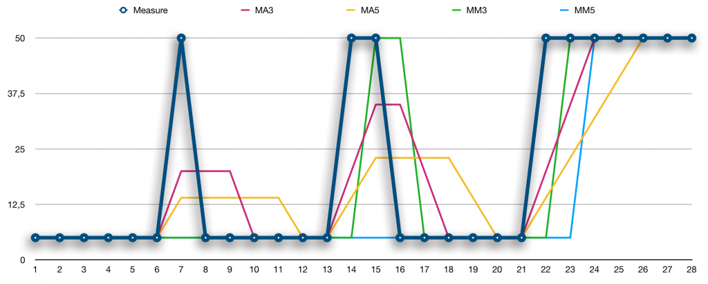
If this is to be done, normal must be what we compare a current value to. A common indicator used for this purpose within daytrading is the moving average. Usually, this is average is windowed over quite a large number of measurements, such as the popular MA50 (last 50 measurements) and MA200 (last 200 measurements), which when they cross is a common trading signal. Moving averages have some downsides though and large windows do too. Let us look at a comparison of four different ways to describe normal, using MA3, MA5, MM3, and MM5, where MM are moving medians, taken on measures that alternate betweeen two values, 5 and 50, over time.

Looking at point 7 in the series, both MAs are disturbed by the peak, whereas both MMs remain at the value 5. Comparing 50 to either of the MMs or MAs would likely lead you to the conclusion that 50 is out of the ordinary, but the MMs are spot on when it comes to what is normal. What is worse is when we reach point 8. Clearly 5 is normal compared to the MMs, but the disturbances of the MAs are still lingering, so it is now difficult to say whether 5 is out of the ordinary or not. Comparing MA3 to MA5, it is obvious that a larger window will reduce the disturbance, but at the cost of extending the lingering.

Moving on to point 14 and 15, two consecutive highs, the MM3 will already at point 15 see the value 50 as the new normal, whereas MM5 will stay at 5. For MMs, the window size determines how many points out of the ordinary are needed for them to become the new normal. Quoting Ian Fleming’s Goldfinger: “Once is happenstance. Twice is coincidence. Three times is enemy action”, he has obviously adopted MM5, as seen in point 24. If we considered using MAs and extending the window size, thinking that the lingering is not too high a price to pay, another issue is seen in points 24 and 26. For MA3 it takes three points to adjust to the new normal and for MA5 it takes five points. The MMs move quicker. For these reasons, MMs will be used as the basis for describing normal behaviour.

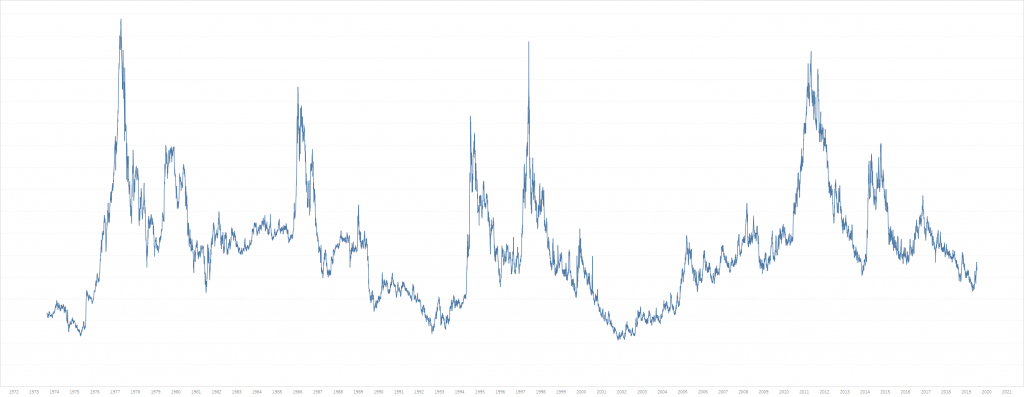
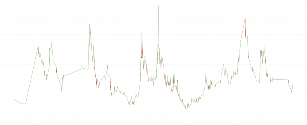
To try things out, let’s see how hard it would be to use this to condense 45 years of daily coffee prices. Coffee is one of the most volatile commodities you can trade, and there has been some significant ups and downs over the years. The data is kindly provided by MacroTrends and a graph can be seen below.

Condensing that will be much harder than the SNMP data, which is tremendously less volatile. The table holding the data is structured as follows:

create table #timeseries (
  Classification char(2), 
  Timepoint date,
  Measure money,
  primary key (
    Classification,
    Timepoint desc
  )
);

Classification is here a two letter acronym making it possible to store more than just coffee (KC) prices. In the case of SNMP data, each device would have it’s corresponding Classification, so you can keep track of each individual time series. For a large network, there could be millions of time series to condense.

In a not so distance past a windowed function that can be used to calculate medians was added to SQL Server, the PERCENTILE_CONT. Unlike many other windowed functions, it does, however and sadly, not allow you specify a window size using ROWS/RANGE. We would want to specify such a size, such that the median is only calculated over the last N timepoints, as in MM3 and MM5 above. As it turns out, with a bit of trickery, it is possible to design your own window. This trick is actually useful for every aggregate that does not support the specification of a window size.

select distinct
  series.Classification,
  series.Timepoint,
  series.Measure,
  percentile_cont(0.5) within group (
    order by windowed_measures.Measure
  ) over (
    partition by series.Classification, series.Timepoint
  ) as MovingMedian
into 
  #timeseries_with_mm
from 
  #timeseries series
cross apply (
  select 
    Measure
  from 
    #timeseries window
  where 
    window.Classification = series.Classification
  and
    window.Timepoint <= series.Timepoint
  order by 
    Classification, Timepoint desc
  offset 0 rows
  fetch next @windowSize rows only
) windowed_measures;

Thanks to the cross apply fetching a specified number of previous rows for every Timepoint the median can be calculated as desired. If @windowSize is set to 3 we get MM3 and with 5 we get MM5. The PERCENTILE_CONT is partitioned so that we calculate the median for every Timepoint. Some rows from the #timeseries_with_mm table are shown in the table below, using MM3.

Classification Timepoint   Measure  MovingMedian
KC             1973-08-20  0,6735   0,6735
KC             1973-08-21  0,671    0,67225
KC             1973-08-22  0,658    0,671
KC             1973-08-23  0,6675   0,6675
KC             1973-08-24  0,666    0,666
KC             1973-08-27  0,659    0,666
KC             1973-08-28  0,64     0,659

Given this, comparisons can be made between a Measure and its MM3. It is possible to settle here, with some threshold for how big a difference should trigger the “out of the ordinary” detection. But, looking at the SNMP data, it’s sometimes affected by low level noise, and similarly Coffee prices have periods of higher volatility. If those, too, are normal, the detection must be fine tuned to not trigger unnecessarily often. To adjust for volatility it is possible to use the standard deviation, corresponding to the STDEVP function in SQL Server. When the volatility becomes higher the standard deviation becomes larger, so we can use this in our detection to be more lenient in periods of high volatility.

select 
  series.Classification,
  series.Timepoint,
  series.Measure,
  series.MovingMedian,
  avg(windowed_measures.MovingMedian) 
    as MovingAverageMovingMedian,
  stdevp(windowed_measures.MovingMedian) 
    as MovingDeviationMovingMedian
into
  #timeseries_with_mm_ma_md
from 
  #timeseries_with_mm series
outer apply (
  select
    MovingMedian
  from
    #timeseries_with_mm window
  where
    window.Classification = series.Classification
  and
    window.Timepoint <= series.Timepoint
  order by
    Classification, Timepoint desc
  offset 1 rows 
  fetch next @trendPoints rows only
) windowed_measures
group by
  series.Classification,
  series.Timepoint,
  series.Measure,
  series.MovingMedian;

I am going to calculate the deviation not over the Measures, but over the MovingMedian, since I want to estimate how noisy the normal is. In this case I will base it on the three previous MM3 values (offset 1 and @trendPoints = 3 above). The reason for not using the current MM3 value is that it is possibly “tainted” by having included the current Measure when it is calculated. What we want is to compare the current Measure with what was previously normal, in order to tell if it’s an outlier. At the same time, it would be nice to know if Measures are trending in some direction, so once we are at it, a moving average of the three previous MM3 values is calculated. As seen above, the window trick can be used in conjunction with GROUP BY as well.

Note that three previous MM3 values require 6 previous Measures to be fully calculated. This means that in daily operations, such as for SNMP data, at least six measures must be kept to perform all calculations, but for each device the seventh and older measures can be discarded. Provided that the older measures can be condensed, this will save a lot of space.

With the new aggregates in place, left to determine is how large the fluctuations may be, before we consider them out of the ordinary. This definitely will take some tweaking, depending on your sources producing the measures, but for the Coffee prices we will settle with the following. Anything within 3.0 standard deviations is considered a non-event. In the rare case that the standard deviation is zero, which can happen if the previous three MM3 values are all equal, we circumvent even the smallest change to trigger an event by also allowing anything within 3% of the moving average. Using these, a tolerance band is calculated and a Measure outside it is deemed out of the ordinary.

-- accept fluctuations within 3% of the average value
declare @averageComponent float = 0.03; 
-- accept fluctuations up to three standard deviations
declare @deviationComponent float = 3.0; 

select 
  Classification,
  Timepoint,
  Measure,
  Trend,
  case 
    when outlier.Trend is not null
    then (Measure - MovingMedian) / (Measure + MovingMedian)
  end as Significance,
  margin.Tolerance,
  MovingMedian
into
  Measure_Analysis
from 
  #timeseries_with_mm_ma_md
cross apply (
  values (
    @averageComponent * MovingAverageMovingMedian + 
    @deviationComponent * MovingDeviationMovingMedian
  )
) margin (Tolerance)
cross apply (
  values (
    case 
      when Measure < MovingMedian - margin.Tolerance then '-'
      when Measure > MovingMedian + margin.Tolerance then '+'
    end 
  )
) outlier (Trend)
order by
  Classification, 
  Timepoint desc;

If the Measure is larger, the trend is positive and negative if it is lower. Events that are deemed out of the ordinary may be so by a small amount or by a large amount. To determine the magnitude of an event, we will use the CHOAS metric. It provides us with a number that becomes larger (positive or negative) as the difference between the Measure and the MovingMedian grows.

Finally, keep the rows that are now marked as outliers (Trend is positive or negative) along with the previous row and following row. The idea is to increase the resolution/granularity around these points, and skip the periods of normality, replacing these with inbound and outbound values.

select
  Classification,
  Timepoint,
  Measure,
  Trend,
  Significance
into
  Measure_Condensed
from (
  select 
    trending_and_following_rows.Classification, 
    trending_and_following_rows.Timepoint, 
    trending_and_following_rows.Measure,
    trending_and_following_rows.Trend,
    trending_and_following_rows.Significance
  from 
    Measure_Analysis analysis
  cross apply (
    select 
      Classification, 
      Timepoint, 
      Measure,
      Trend,
      Significance
    from 
      Measure_Analysis window
    where
      window.Classification = analysis.Classification
    and
      window.Timepoint >= analysis.Timepoint 
    order by
      Classification,
      Timepoint asc
    offset 0 rows
    fetch next 2 rows only
  ) trending_and_following_rows
  where 
    analysis.Trend is not null
  union
  select 
    trending_and_preceding_rows.Classification, 
    trending_and_preceding_rows.Timepoint, 
    trending_and_preceding_rows.Measure,
    trending_and_preceding_rows.Trend,
    trending_and_preceding_rows.Significance
  from 
    Measure_Analysis analysis
  cross apply (
    select 
      Classification, 
      Timepoint, 
      Measure,
      Trend,
      Significance
    from 
      Measure_Analysis window
    where
      window.Classification = analysis.Classification
    and
      window.Timepoint <= analysis.Timepoint 
    order by
      Classification,
      Timepoint desc
    offset 0 rows
    fetch next 2 rows only
  ) trending_and_preceding_rows
  where 
    analysis.Trend is not null
  union
  select
    analysis.Classification,
    analysis.Timepoint,
    analysis.Measure,
    analysis.Trend,
    analysis.Significance
  from (
    select
      Classification,
      min(Timepoint) as FirstTimepoint,
      max(Timepoint) as LastTimepoint
    from
      Measure_Analysis
    group by
      Classification 
  ) first_and_last
  join
    Measure_Analysis analysis
  on
    analysis.Classification = first_and_last.Classification
  and
    analysis.Timepoint in (
      first_and_last.FirstTimepoint, 
      first_and_last.LastTimepoint
    )
) condensed;

The code needs to manage the first and last row in the timeseries, which may not be trending in either direction, but needs to be present in order to produce a nice graph. This will reduce the Coffee prices table from 11 491 to 884 rows. That this was harder than for SNMP data is shown by the “compression ratio”, which in this case is approximately 1:10, but for SNMP reached 1:1000. The condensed graph can be seen below.

Colors are deeper red for negative Significance and deeper green for positive Significance. What is interesting is that Coffee seems to have periods that are uneventful and other periods that are much more eventful. These periods last years. Of course, trading is more fun when the commodity is eventful, and unfortunately it seems as if we are in an uneventful period right now.

In this article, code has been optimized for readability and not for performance. Coffee may not have been the best example from a condensability perspective, but it has some interesting characteristics and its price history is freely available. There are surely other ways to do this and the method presented here can likely be improved, so I would be very happy to receive comments along those lines.

The complete code can be found by clicking here.